Spectral Permutation Demo

Importing Packages

import numpy as np
import pandas as pd
from mheatmap import (
    amc_postprocess,  
    mosaic_heatmap
)
from mheatmap.graph import spectral_permute
from mheatmap.constants import set_test_mode

set_test_mode(True)

import matplotlib.pyplot as plt
import scipy

Load Data

Load the ground truth labels
- Salinas_gt.mat: Ground truth labels for Salinas dataset
Load the predicted labels from spectral clustering

# Load the data
y_true = scipy.io.loadmat("data/Salinas_gt.mat")["salinas_gt"].reshape(-1)
# Load predicted labels from spectral clustering
y_pred = np.array(
    pd.read_csv(
        "data/Salinas_spectralclustering.csv",
        header=None,
        low_memory=False,
    )
    .values[1:]
    .flatten()
)
print(f"y_true shape: {y_true.shape}")
print(f"y_pred shape: {len(y_pred)}")

y_true shape: (111104,)
y_pred shape: 111104

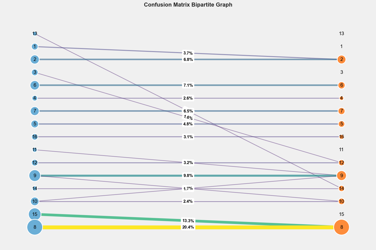
AMC Post-processing

Alignment with Hungarian algorithm
Masking the zeros (unlabeled pixels) with mask_zeros_from_gt
Computing the confusion matrix

See AMC Post-processing for more details.

# AMC post-processing
_, conf_mat, labels = amc_postprocess(y_pred, y_true)

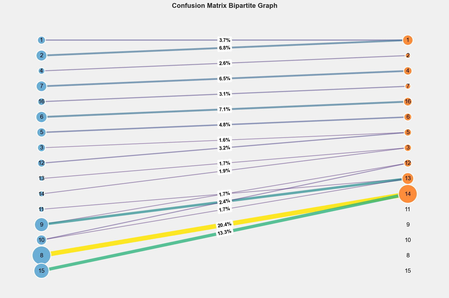
Spectral Permutation

Treat the confusion matrix as an adjacency matrix

\[ A = C \]

Compute the graph Laplacian

\[ L = D - A \]

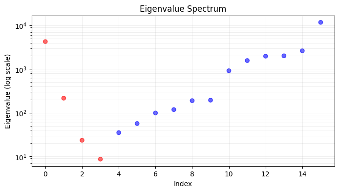
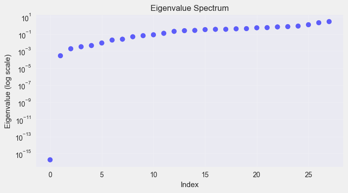
Compute the eigenvectors and eigenvalues

\[ L = U \Sigma U^T \]

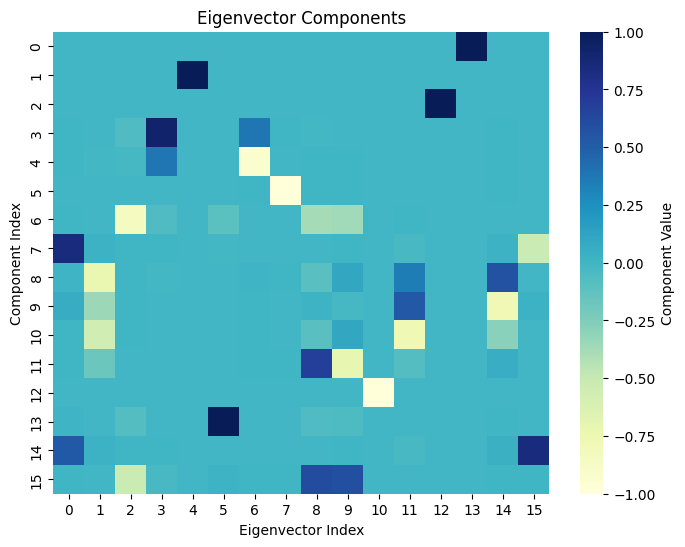
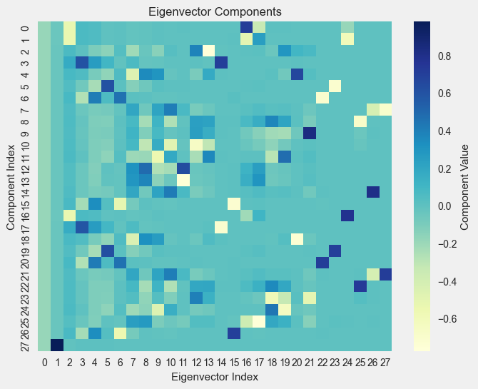
Sort the eigenvectors based on the eigenvalues

\[ U = [u_1, u_2, \ldots, u_n] \]

Fiedler vector is the second smallest eigenvector

\[ f = u_2 \]

Sort the labels based on the Fiedler vector

\[ \pi\tilde{y} = \tilde{y}[f] \]

Reorder the confusion matrix based on the sorted labels

\[ \pi C = C[f, f] \]

# spectral reordering
reordered_mat, reordered_labels = spectral_permute(conf_mat, labels)

png png png

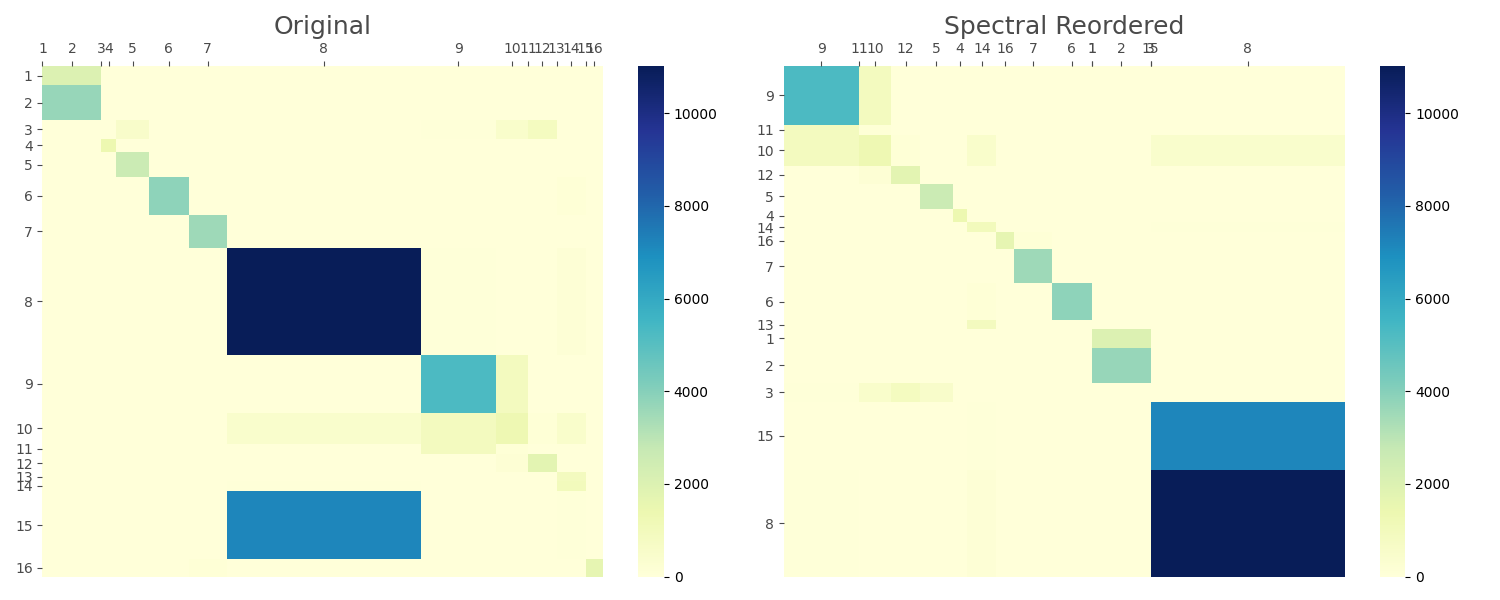
Visualize the Results

# Visualize original vs spectrally reordered matrices
fig, (ax1, ax2) = plt.subplots(1, 2, figsize=(15, 6))

mosaic_heatmap(conf_mat, ax=ax1, xticklabels=labels, yticklabels=labels, cmap="YlGnBu")
ax1.set_title("Original", fontsize=18, color='#4A4A4A')  # Medium gray
ax1.xaxis.set_ticks_position('top')
ax1.tick_params(colors='#4A4A4A')

mosaic_heatmap(
    reordered_mat,
    ax=ax2,
    xticklabels=reordered_labels,
    yticklabels=reordered_labels,
    cmap="YlGnBu",
)
ax2.set_title("Spectral Reordered", fontsize=18, color='#4A4A4A')  # Medium gray
ax2.xaxis.set_ticks_position('top')
ax2.tick_params(colors='#4A4A4A')

plt.tight_layout()
plt.show()

png

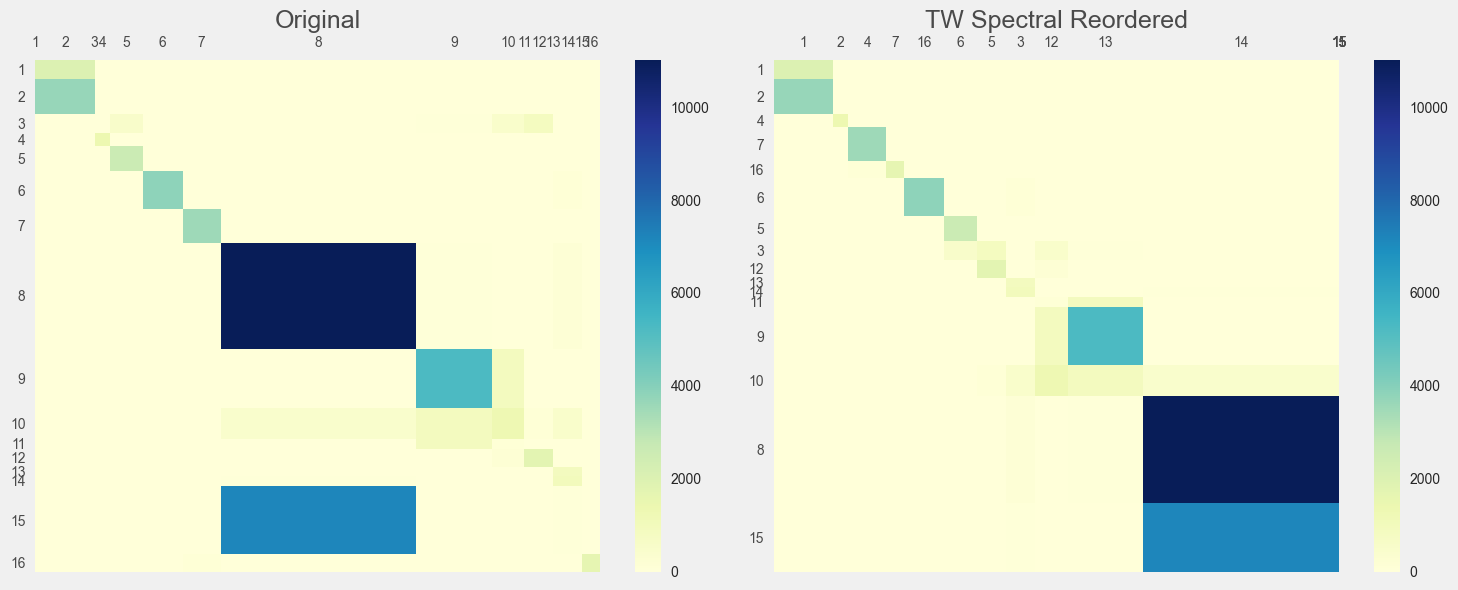
Two-walk Spectral Permutation

# Two-walk Laplacian
reordered_mat, reordered_labels = spectral_permute(conf_mat, labels, mode='tw')

png png png

Visualize the TW Results

# Visualize original vs spectrally reordered matrices
fig, (ax1, ax2) = plt.subplots(1, 2, figsize=(15, 6))

mosaic_heatmap(conf_mat, ax=ax1, xticklabels=labels, yticklabels=labels, cmap="YlGnBu")
ax1.set_title("Original", fontsize=18, color='#4A4A4A')  # Medium gray
ax1.xaxis.set_ticks_position('top')
ax1.tick_params(colors='#4A4A4A')

mosaic_heatmap(
    reordered_mat,
    ax=ax2,
    xticklabels=reordered_labels,
    yticklabels=reordered_labels,
    cmap="YlGnBu",
)
ax2.set_title("TW Spectral Reordered", fontsize=18, color='#4A4A4A')  # Medium gray
ax2.xaxis.set_ticks_position('top')
ax2.tick_params(colors='#4A4A4A')

plt.tight_layout()
plt.show()

png